How to use the Amnis ImageSteamX MkII
Jump to:
Start up the ImageStream
Check the reagents. Open the door in front of the instrument and refill the reagents and/or empty the waste.

Reagents:
The following table gives information about the reagents. To refill the bottles of reagents, unscrew the lid carefully. The lid is attached to the instrument. You can only transfer the bottle without the lid.
Cleanser, debubbler and steriliser are located in the cupboard in the flow facility room.

Waste container:
The waste bottle holds all of the fluids that have been run through the ImageStream®X MkII, and can hold up to 1600 mL. If the waste container is full, push on the quick-disconnect buttons to remove the tubing from the Waste tank. Keep in mind these lines are attached to the instrument. Take the bottle and empty it carefully down the sink (wearing PPE). Add approx. 160 mL of bleach to the empty bottle. It is recommended that the waste bottle contain 10% bleach when full.
SpeedBeads:
If the speed beads are not enough to run your experiment, replace them with a new tube. There are spare in the fringe in the flow facility room.

2. Turn on the instrument by pressing the 3 buttons as shown in the following picture. (left to right)

3. Log on:
user name: Amnis
password: is100
4. Launch the INSPIRE software by double-clicking the INSPIRE icon on the desktop.

5. Click Startup.

This script fills the system with sheath and flushes out all of the old sheath or rinse that was in the system. The sample line is prepared by loading 50 µL of air into the uptake line. Beads are loaded into the bead pump from the 15 mL conical tube. The Initializing Fluidics window opens, showing the progress bar.

6. When calibrations and tests finish, a window appears as the following:
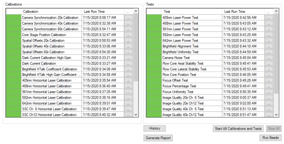
7. If a calibration or test fails (red colour instead of green), run that calibration or test individually by clicking on the failed calibration or test. If it fails again, please contact Flow facility team.
NOTE: The whole procedure of starting up takes about 45 mins.
Setting up an experiment
Adjusting the settings
On the right hand side of the screen, select the settings of the experiment.
File acquisition:

Enter the file name in the Filename field.
Enter the sequential number in the Seq # field.
NOTE: The sequential number is appended to the file name, followed by the .rif or .fcs extension. The sequence number increases by 1 with each successive data acquisition. Files collected with BF off will be appended with "noBF," and files collected with EDF enabled will be appended with "EDF" in the file names.
Click the folder icon to select a folder where data acquisition files will be saved. You can also create a new folder to save acquisition files in.
Enter the number of cells you want to acquire in the Count field and select the population from the adjacent dropdown. To count one population but limit the collection to another population, click on the bracket to break the link and enable the Collect drop-down.
Illumination:

Click on the laser buttons to turn on each laser used in the experiment. When they turn light blue, they are on.
To select the channels, click on a channel name to open the Channel Selection window.

Select the box next to the channel name to enable collection of the specified channel. When you have selected all channels to be collected, click OK.

NOTE: Select Brightfield channels (Ch1 and 9) and SSC (Ch6)
Magnification & EDF:

Choose the objective under Magnification
Select the EDF checkbox if you want extended depth of field (EDF) collection.
Fluidics:

Click ‘STOP’ to prematurely stop acquisition. The system prompts you to either discard the acquired data or to save the collected data in a file.
Click ‘PAUSE’ to pause acquisition while running or to resume acquisition when paused.
Click ‘RUN’ to continue the acquisition.
Set the speed from Low to High. The table below shows the pixel resolution, relative sensitivity and approximate time to collect 10,000 objects at a concentration of 1 x 10⁷objects per ml at different magnifications and speed settings. In order to run at a higher speed, the rows on the camera are binned, this means the signal is collected in 1, 2 or 4 rows of the CCD at a time.

NOTE: Binning refers to the number of pixel rows used to collect the data.
Focus and centering:

Center the core stream images (if necessary) by laterally moving the objective under Focus and Centering. Adjust centering by pressing the right or left arrows.
The table below explains the Analysis Area Tools:

The table below explains The Image gallery:

Running a sample
Using eppendorfs (this is the type of tube the instrument can get)
Press Load and load an aliquot of the brightest sample in the experiment that fluoresces with each fluorochrome used. It is critical that you run this sample first to establish the instrument settings.
NOTE: DO NOT change laser settings for the experiment once established on this sample.
When prompted, place sample vial with 20-200 μL into the sample loader.

Click Acquire to begin acquiring a data file. The data file(s) are automatically saved in the selected folder once the desired number of objects are collected.
During acquisition, you might need to adjust the display settings.
Click on the Display Settings tool to open the window.
Select the channel by clicking on the channel name.
To change the channel name, type a new name. To change the channel colour, click on the colour box.
To set the display mapping, adjust the right and left green bars in the graph. You will adjust the Display Intensity settings on the graph (the Y Axis) to the Pixel Intensity (the X axis). The range of pixel intensities is 0-4095 counts. The display range is 0–255. The pixel intensities shown in grey are gathered from the images coming through in the specific channel and updates with every 10 images. Updates to the adjustments can be visualized in the image gallery. At each intensity on the X Axis of the graph, the grey histogram shows the number of pixels in the image. This histogram provides you with a general sense of the range of pixel intensities in the image. The dotted green line maps the pixel intensities to the display intensities, which are in the 0–255 range.
Click and drag the vertical green line on the left side (crossing the X Axis at 0) to manually set the display pixel intensity to 0 for all intensities that appear to the left of that line. This removes background noise from the image.
Click and drag the vertical green line on the right side to set the display pixel intensity to 255 for all intensities that appear to the right of that line.

Create graphs to gate on cells of interest.
To create graphs:
From analysis area tools, select one of these two icons (histogram or dot plot)

For dot plots, the New Scatterplot window will appear:

- Type the title of the graph and select X axis and Y axis feature from the drop down menu. Click OK.
- Create a dot plot Area vs Aspect Ratio. Gate on cells to eliminate debris and doublets. Single cells will have an intermediate Area value and a high Aspect Ratio. For example:

- Create a new histogram, as in picture below:

- Gate on cells that are best in focus. To rename the gate, you need to type the name on the window that appears after you create the gate.

- The cells with better focus have higher Gradient RMS, values. Begin your region at the bin after the Gradient RMS value you wish to exclude and continue the region to the maximum in the plot. For example:

Tools on the graph window explained below:

Once acquisition finishes, either load the next sample or return the remaining sample.

NOTE: If the next sample has no nuclear dye and follows a DNA intercalating dye-stained sample, load a solution of 10% bleach and then load PBS to ensure that residual dye does not stain the subsequent samples.
Change the file name for the next sample and continue collecting samples until you have acquired data for all the desired samples.
When finished running the experiment samples or after setting the template, run single colour compensation controls.
Click in the analysis tools section and choose Compensation to launch the Compensation Wizard.
NOTE: The Compensation Wizard sets the instrument for compensation controls that must be collected with brightfield and scatter (785 nm laser) OFF and every channel set to be collected. Keep all laser powers the same as for the experimental samples.
Follow the prompts in the Compensation Wizard to collect all compensation control files:
a. Click Load. Alternately, if a compensation control sample is already running, click Next.
b. Place the tube on the uptake port and click OK.
c. Click Next when sample is running.
d. Verify the channel for compensation.
e. If not all cells are positive, draw a region on the Uncompensated Intensity scatter plot to define the positive population. View the population in the Image Gallery and choose this population to collect.
f. Name the file and choose the path to save the data.
g. Click Collect File. The compensation coefficients are calculated. The compensation coefficients and an Intensity scatter plot using the coefficients displays.
h. Click OK on the Acquisition Complete popup window.
i. Click Load to continue with the next single colour control sample or click Return (optional).
j. Repeat the previous steps for each compensation sample. For each sample, reset the Image gallery population to view All, then create an appropriate population for each sample.
NOTE: The R1 gate can be moved for each sample.
k. Click Exit when done with the Compensation Wizard.
Save the coefficients to a compensation matrix file. The beginning template is restored and the saved matrix is used to compensate the Intensity feature.
Using plates
To run a plate:
Go to ‘Autosampler’ tab.
Choose ‘Define plate’

NOTE: There is the option to run the sample of one well only. You can do that before running the plate, so you can create a template you will further apply on the plate.
To do that
Go to ‘Autosampler’ tab and select ‘Load from well’.
Save this as template.
Well definition window will open:

Create a new definition. Alternately, click the folder icon to browse for a previously saved definition to edit.
Name the plate definition.
NOTE: At a minimum, each well requires an Output File Path, Max Acquisition Time, and Template File in order to be considered "defined". Other parameters can be added to the definition in the next step.
Choose the parameters you would like to use. Click Add/Remove Well Parameters to choose the parameters you want to report for the wells
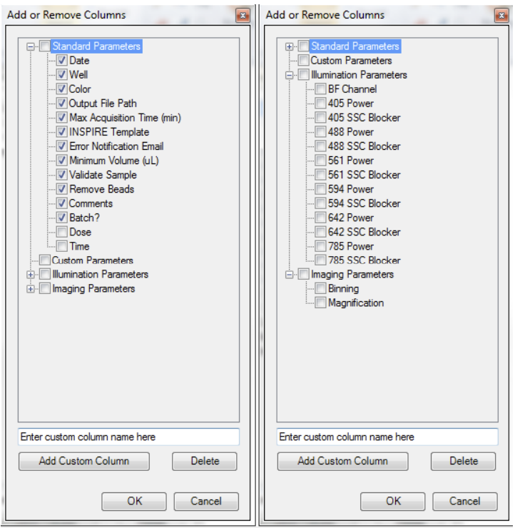
There are several categories of parameters that may be chosen as a group or individually. See the list of parameters above. Check or uncheck the desired parameters. The user can also define custom parameters. Expand the category to see the individual parameters. To delete a custom parameter, select it and use the delete key. Click OK when done.
NOTES:
- It is highly recommended to leave the Validate Sample option 'Yes'.
- To include a parameter in the file name, click in the box below the column heading (make sure it says ‘yes’).
- Columns can be re-ordered by click/drag.
- Batching of the data into IDEAS may be done if a compensation matrix and template exist for the experiment.
- Click OK when finished adding or removing parameters.
Define the wells. Select wells to define by clicking
a) individually (or Ctrl click / shift click for multi-select),
b) rows or columns,
c) colour,
d) the ‘Select Defined’ button or
e) All.
In this example column 1 is selected.

You can edit values for some of the Custom and many of the Standard parameters. You can do this for all selected wells or for individual wells.
For example, if you want to collect with Max Acquisition Time 10 minutes for the selected wells, type 10 in the 'Apply to selected' box below the Max Acquisition Time heading. If you want to only apply this to a single well, type this value in the box corresponding to that well.

Click ‘Save’.
Click ‘Start’ to run the plate. The Auto Sampler Unattended Operation window opens with the Plate Definition you just saved. If you wish to choose a different Plate Definition, browse for it by clicking on the folder icon. l If you want to edit the Plate Definition, click Edit and you will be taken to the Well Plate Definition window.

Check or uncheck the boxes Return samples, Sterilize, Shutdown.
NOTE: Note that these boxes may be checked or unchecked while the plate is running and the operation will apply after the current sample is finished.
Select the wells to run (they will appear in the list).
Click ‘Eject Tray’ to extend the plate nest.
Add at a minimum 75 μL samples to the 96 well plate, cover with Sigma-Aldrich X-Pierce Film (XP-100, Cat # 2722502) to minimize evaporation and allow the membrane piercing probe to access the sample. Place your plate on the tray with well A1 positioned at the upper left corner.
Click Start to begin.
The Status column will be updated for each well as it is run. For each sample, the instrument performs the following in sequence: 1) Mixing and resuspension of sample, 2) Load, 3) Validation (flow speed CV, focus, brightfield intensity, object rate), 4) Data Acquisition, 5) Result(success or error).
Shut Down
If you are the last person who uses the instrument for the day, please shut down the system following the procedure below:
This procedure sterilizes the ImageStream®X MkII system and leaves it with pumps empty and water in the fluidic lines.
The instrument is left on with INSPIRE running.
Fill the Rinse, Cleanser, Sterilizer, and Debubbler bottles if necessary.
Empty the Waste bottle.
Remove any tubes from the uptake ports.
Click Shutdown (bottom right on the screen)

NOTE: This procedure automatically turns off all illumination sources and rinses the entire fluidic system with deionized (DI) water, sterilizer, cleanser, de-bubbler, and then water again. The sterilizer is held in the system for ten minutes to ensure de-contamination. It takes about 45 minutes of unattended (walk-away) operation to complete.
If someone has booked the instrument after you, please leave the INSPIRE running and clear the compensation matrix.

Troubleshooting
Unstable fluidics
Possible cause: Air bubbles or clog in system.
Recommended solution:
1. Go to ‘Instrument’ tab and select ‘purge sample line’
2. When this is done, select ‘sterilise line’
3. Then select ‘Prime’
4. When it is finished, select ‘Purge bubbles’
5. If nothing from above works, do a ‘start up’ again.
Cross-contamination from previous samples
Possible cause: Residues (cells or DNA dye) from previous samples appear in current sample
Recommended solution:
1. Load a sample of 10% bleach and run for 20mins.
2. Load a sample of PBS and run for 20mins
Instrument fails in test(s) after ‘Start up’
Recommended solution:
1. Click on the failed test and rerun
2. If it still fails, contact Facility Team
Software fails to launch
Possible cause: Loss of communication between the computers and instrument.
Recommended solution:
1. Shut down the computer
2. power off the instrument.
3. Power on the instrument and the computer, wait 5 min and try launching INSPIRE™.